Blackbody Radiation and the Quantum Revolution
The Blackbody Problem
A blackbody is an ideal system that absorbs all incident electromagnetic radiation. When it is in thermal equilibrium, the radiation it emits has a spectrum determined only by its temperature. The spectrum is therefore independent of the chemical composition of the walls used to produce it.
During the nineteenth century, this universality made blackbody radiation a central problem in thermodynamics and electromagnetic theory. Classical physics accounted for parts of the observed spectrum, but its general prediction failed at high frequencies. Planck’s solution introduced discrete energy elements and became one of the first steps toward quantum theory.
Kirchhoff’s Law and the Cavity Model
For a body at temperature $T$, let $e_\nu$ denote its spectral emissive power and $a_\nu$ its absorptivity at frequency $\nu$. Kirchhoff showed that, at thermal equilibrium, the ratio
\[\frac{e_\nu}{a_\nu}\]is a universal function of $\nu$ and $T$. A perfect absorber has $a_\nu=1$, so its emission provides the universal equilibrium spectrum directly.
A physical approximation is obtained with a cavity whose walls are maintained at a fixed temperature and which communicates with the exterior through a small hole. Radiation entering the hole undergoes many reflections and has a high probability of being absorbed. The radiation emerging from the same hole is determined mainly by the equilibrium field inside the cavity. This construction separates the universal spectrum from the properties of a particular surface.
Energy Density and Spectral Distribution
Let $u(T)$ be the electromagnetic energy per unit volume inside the cavity. The spectral energy density per unit frequency, denoted by $u_\nu(T)$, is defined by
\[du=u_\nu(T)\,d\nu.\]Its units are
\[\left[u_\nu\right] = \frac{\mathrm J}{\mathrm{m}^3\,\mathrm{Hz}}.\]The total energy density is obtained by integrating over all positive frequencies:
\[u(T)=\int_0^\infty u_\nu(T)\,d\nu.\]The same spectrum can be described per unit wavelength. Since
\[\nu=\frac{c}{\lambda},\]the two densities must satisfy
\[u_\lambda(T)\,d\lambda = -u_\nu(T)\,d\nu.\]Taking absolute values of the differential gives
\[u_\lambda(T) = u_\nu(T)\left|\frac{d\nu}{d\lambda}\right| = \frac{c}{\lambda^2} u_\nu(T).\]This factor is essential. A spectral density is defined relative to an interval, and equal intervals of frequency do not correspond to equal intervals of wavelength. The maximum of $u_\nu$ therefore does not transform into the maximum of $u_\lambda$ simply through $\nu=c/\lambda$.
Wien’s and Stefan-Boltzmann Laws
Before Planck’s complete formula, thermodynamics already imposed important restrictions on the spectrum. Wien’s displacement law states that the wavelength at which $u_\lambda(T)$ reaches its maximum satisfies
\[\lambda_{\max}T=b,\]where $b$ is Wien’s displacement constant. Increasing the temperature shifts the maximum of the wavelength spectrum toward shorter wavelengths.
The total energy density is proportional to the fourth power of the absolute temperature:
\[u(T)=aT^4.\]For the radiant exitance $M$, the corresponding Stefan-Boltzmann law is
\[M=\sigma T^4.\]These results describe the position of the maximum and the total emitted energy, while leaving the complete spectral distribution to be determined.
The Classical Prediction
Electromagnetic waves in a cavity can be decomposed into normal modes. The number of modes per unit volume in the interval between $\nu$ and $\nu+d\nu$ is
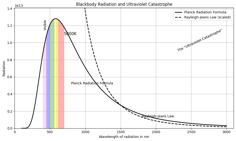
\[g(\nu)\,d\nu = \frac{8\pi\nu^2}{c^3}\,d\nu.\]Classical statistical mechanics assigns an average energy $kT$ to each mode through the equipartition theorem. Multiplying the density of modes by this average energy gives the Rayleigh-Jeans law:
\[u_\nu^{\mathrm{RJ}}(T) = \frac{8\pi\nu^2kT}{c^3}.\]At low frequencies this formula agrees with observation. At high frequencies it grows as $\nu^2$. Integrating it over all frequencies gives
\[\int_0^\infty u_\nu^{\mathrm{RJ}}(T)\,d\nu = \infty.\]The divergence became known as the ultraviolet catastrophe. It does not describe an experimentally observed release of infinite energy; it shows that the combination of classical mode counting and equipartition cannot represent the equilibrium spectrum at all frequencies.
Planck’s Hypothesis
Planck modeled the exchange of energy between the electromagnetic field and resonators in the cavity walls. For a resonator of frequency $\nu$, he introduced discrete energy values
\[E_n=nh\nu, \qquad n=0,1,2,\ldots,\]where $h$ is Planck’s constant.
The Boltzmann factor assigns the level $E_n$ a weight proportional to
\[e^{-E_n/(kT)} = e^{-nh\nu/(kT)}.\]The partition sum is the geometric series
\[Z = \sum_{n=0}^{\infty} e^{-nh\nu/(kT)} = \frac{1} {1-e^{-h\nu/(kT)}}.\]The average energy of a resonator is
\[\overline E = -\frac{\partial}{\partial\beta}\ln Z, \qquad \beta=\frac{1}{kT},\]and therefore
\[\overline E = \frac{h\nu} {e^{h\nu/(kT)}-1}.\]Unlike the classical value $kT$, this average energy decreases exponentially when $h\nu$ is large compared with $kT$. High-frequency modes are consequently suppressed.
Planck’s Radiation Law
Multiplying the density of electromagnetic modes by the average energy gives Planck’s law in frequency form:
\[u_\nu(T) = \frac{8\pi h\nu^3}{c^3} \frac{1} {e^{h\nu/(kT)}-1}.\]Using the change of variable between frequency and wavelength gives
\[u_\lambda(T) = \frac{8\pi hc}{\lambda^5} \frac{1} {e^{hc/(\lambda kT)}-1}.\]The two formulas describe the same radiation field through different spectral variables. Their graphs have different maxima because the density changes under the transformation from $\nu$ to $\lambda$.
Planck’s constant is
\[h = 6.62607015\times10^{-34}\ \mathrm{J\,s}.\]In Planck’s original argument, discreteness concerned the energy exchanged by the resonators. The interpretation of light itself in terms of quanta was developed more explicitly by Einstein in 1905.
Classical Limits of Planck’s Law
For low frequencies,
\[h\nu\ll kT,\]the exponential can be expanded:
\[e^{h\nu/(kT)} \approx 1+\frac{h\nu}{kT}.\]Planck’s law then becomes
\[u_\nu(T) \approx \frac{8\pi\nu^2kT}{c^3},\]which is the Rayleigh-Jeans law.
For high frequencies,
\[h\nu\gg kT,\]the denominator is approximately $e^{h\nu/(kT)}$, and
\[u_\nu(T) \approx \frac{8\pi h\nu^3}{c^3} e^{-h\nu/(kT)}.\]This is Wien’s high-frequency form. Planck’s expression therefore contains the successful limiting results while avoiding the classical divergence.
From a Spectral Problem to Quantum Theory
The blackbody problem did not arise because classical physics lacked equations for radiation. The difficulty came from applying classical statistical assumptions to the electromagnetic modes of a cavity. Mode counting produced the factor $\nu^2$; equipartition assigned the same mean energy $kT$ to every mode; together they led to a divergent spectrum.
Planck changed the statistical distribution of energy by introducing the scale $h\nu$. The agreement with the observed spectrum showed that this modification could not be confined to a numerical correction. It required a different account of the relation between matter, radiation, and energy exchange, which subsequent developments transformed into quantum theory.